How Database Indexes Work: B-Tree Pages, Query Plans, and the Write Cost

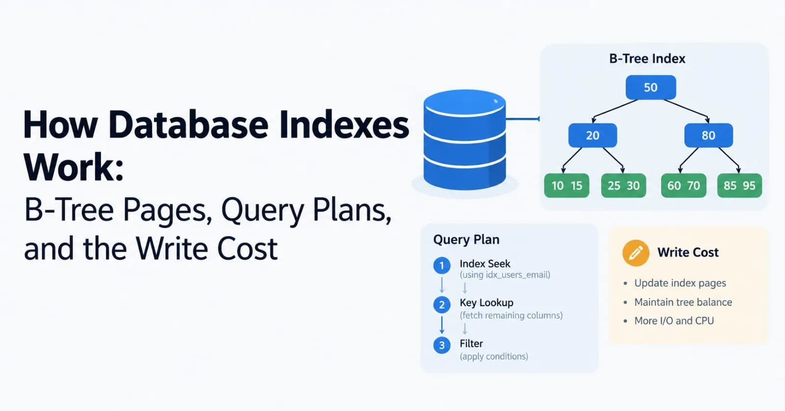
A database index is a separate, sorted structure that maps column values to row locations, so a query can jump to the rows it needs instead of reading the whole table. In the lab built for this post, a PostgreSQL 16.15 table of one million rows answered the same lookup by reading 19,231 buffers without an index and 23 with one. This post shows where that gap comes from using real EXPLAIN output, then covers when an index does not help and what it costs on writes.

Every plan and number below was produced by scripts I ran against a local server, and the SQL is shown inline so you can repeat it. Statements about documented behavior link to the PostgreSQL manual, which is the version 18 manual at the time of writing. The lab itself ran 16.15, and I mark the one place where that difference matters.

The short version

The lab

The table is an orders table with one million rows: a bigint id, a customer_id between 1 and 50,000, a status that is paid for 97% of rows, an email that is unique per row, and a padding column so rows have a realistic width. Rows were inserted in time order, so created_at grows with the physical position of each row.

CREATE TABLE orders (
    id          bigint        NOT NULL,
    customer_id integer       NOT NULL,
    status      text          NOT NULL,
    created_at  timestamptz   NOT NULL,
    email       text          NOT NULL,
    total       numeric(10,2) NOT NULL,
    note        text          NOT NULL
);

SELECT setseed(0.42);

INSERT INTO orders
SELECT i,
       1 + floor(random() * 50000)::int,
       CASE WHEN r < 0.97 THEN 'paid' WHEN r < 0.99 THEN 'pending' ELSE 'failed' END,
       timestamptz '2026-01-01 00:00:00+00' + i * interval '30 seconds',
       'User' || i || '@Example.com',
       round((random() * 500)::numeric, 2),
       repeat(md5(i::text), 2)
FROM (SELECT i, random() AS r FROM generate_series(1, 1000000) AS g(i)) AS s;

ALTER TABLE orders ADD PRIMARY KEY (id);
ANALYZE orders;

The heap is 150 MB spread over 19,231 pages. The server ran with these settings, and everything stayed in cache, so timings reflect CPU and buffer work rather than disk waits. I disabled autovacuum on purpose so the visibility map effect in the covering index section is visible. Leave it on in production.

shared_buffers = 1GB
max_parallel_workers_per_gather = 0
jit = off
fsync = off
autovacuum = off

Timings are noisy, so this post leans on buffer counts, which were identical in every run. The plans below are the first execution of each query in the scripted run, trimmed to the relevant lines, and every query shown here without EXPLAIN was run under EXPLAIN (ANALYZE, BUFFERS, COSTS OFF). Where a table quotes a time, it is the median of nine repeated runs in one session. The unindexed lookup below took 85 ms in the scripted run and a median of 45 ms across nine repeats.

A query with no index

Customer 4242 has 20 orders. With no index on customer_id, PostgreSQL has only one way to find them.

EXPLAIN (ANALYZE, BUFFERS, COSTS OFF) SELECT * FROM orders WHERE customer_id = 4242;

Seq Scan on orders (actual time=4.300..85.046 rows=20 loops=1)
  Filter: (customer_id = 4242)
  Rows Removed by Filter: 999980
  Buffers: shared hit=19231
Planning Time: 0.343 ms
Execution Time: 85.088 ms

The buffer count equals the number of heap pages in the table. The database read every page to return 20 rows and discarded the other 999,980.

The same query with an index

CREATE INDEX orders_customer_id_idx ON orders (customer_id);

Rerunning the same EXPLAIN gives a very different plan. This is the warm second run.

Bitmap Heap Scan on orders (actual time=0.006..0.013 rows=20 loops=1)
  Recheck Cond: (customer_id = 4242)
  Heap Blocks: exact=20
  Buffers: shared hit=23
  ->  Bitmap Index Scan on orders_customer_id_idx (actual time=0.004..0.004 rows=20 loops=1)
        Index Cond: (customer_id = 4242)
        Buffers: shared hit=3
Planning Time: 0.030 ms
Execution Time: 0.021 ms

The 23 buffers split into 3 index pages and 20 heap pages, one per matching row, because the 20 orders sit on 20 different heap pages. That is 836 times fewer buffers than the sequential scan. The index uses exactly 3 pages for this lookup, and the next section shows why.

In PostgreSQL every index is a secondary index stored separately from the table's heap, so an ordinary index scan fetches from both the index and the heap. This plan uses a bitmap scan, which collects matching row locations first and then visits table rows in physical order.

Inside a B-tree index

The default index type is a B-tree, a multi-way balanced tree. Any data type that sorts into a well-defined order can be indexed. Leaf pages hold the sorted keys together with the location of each row, and internal pages hold separator keys that tell a search which child to visit.

flowchart TD
    R["Root page<br/>1 page, 4 downlinks"]
    I1["Internal page"]
    I2["Internal page"]
    I3["Internal page"]
    I4["Internal page"]
    L1["Leaf page<br/>sorted keys + row locations"]
    L2["Leaf page"]
    L3["Leaf page"]
    H["Heap pages<br/>the table rows"]
    R --> I1
    R --> I2
    R --> I3
    R --> I4
    I1 --> L1
    I1 --> L2
    I1 --> L3
    L1 -- "right link" --> L2
    L2 -- "right link" --> L3
    L1 -. "row location" .-> H

PostgreSQL follows the Lehman and Yao design. As its nbtree README explains, each page gets a right link to its right sibling and a high key that bounds the keys allowed on that page. A search that lands on a page that was just split follows the right link, so searches need no locks beyond a short page lock while reading a page.

I measured the shape of the customer_id index with the pageinspect extension.

SELECT level, fastlevel, root FROM bt_metap('orders_customer_id_idx');

SELECT type, count(*) AS pages
FROM generate_series(1, (pg_relation_size('orders_customer_id_idx') / 8192 - 1)::int) AS g(n),
     LATERAL bt_page_stats('orders_customer_id_idx', g.n)
GROUP BY type ORDER BY type;

Level 2 means a lookup visits three pages: the root, one internal page, and one leaf. That matches the Bitmap Index Scan above, which reported exactly 3 buffers. Each internal page fans out to roughly 240 children on average here (969 leaf pages under 4 internal pages), which is why height grows so slowly. The 21 MB primary key index on one million bigints is also only 3 levels deep.

Reading the root page directly shows the separators.

SELECT itemoffset, ctid, itemlen, data
FROM bt_page_items('orders_customer_id_idx', 290) LIMIT 4;

itemoffset |  ctid   | itemlen |          data
------------+---------+---------+-------------------------
          1 | (3,0)   |       8 |
          2 | (289,1) |      16 | 3b 39 00 00 00 00 00 00
          3 | (575,1) |      16 | 8b 72 00 00 00 00 00 00
          4 | (860,1) |      16 | cd ab 00 00 00 00 00 00

The first number in each ctid is the block number of a child page. Read as little-endian integers, the separator keys 3b 39, 8b 72 and cd ab are 14651, 29323 and 43981. They split the customer_id range of 1 to 50,000 into four subtrees. The first item stores no key at all, because it points to the subtree for values below the first separator.

Two storage details explain the sizes in this post. When a page fills, PostgreSQL splits it, and the README says it tries to equalize the number of bytes, not items on each half. And the customer_id index is small because each of the 50,000 values appears about 20 times, and deduplication stores a duplicated key once followed by a sorted array of row locations.

When the planner uses an index

Having an index does not force its use. PostgreSQL uses an index when it thinks that is more efficient than a sequential scan, and it relies on statistics that ANALYZE refreshes. The same engine picked four different scan types in this lab for four different situations.

flowchart LR
    ST["Table statistics<br/>from ANALYZE"] --> EST["Estimated rows<br/>matching the filter"]
    EST --> CAND["Candidate plans<br/>Seq Scan, Index Scan,<br/>Bitmap Heap Scan, Index Only Scan"]
    IDX["Available indexes and<br/>visibility map state"] --> CAND
    CAND --> PICK["Lowest estimated cost wins"]

Selectivity is the first thing that decides. I added an index on status, which holds 970,195 paid rows, 19,854 pending and 9,951 failed.

CREATE INDEX orders_status_idx ON orders (status);
EXPLAIN (ANALYZE, BUFFERS, COSTS OFF) SELECT * FROM orders WHERE status = 'paid';
EXPLAIN (ANALYZE, BUFFERS, COSTS OFF) SELECT * FROM orders WHERE status = 'failed';

Seq Scan on orders (actual time=0.006..91.261 rows=970195 loops=1)
  Filter: (status = 'paid'::text)
  Rows Removed by Filter: 29805
  Buffers: shared hit=19231

Index Scan using orders_status_idx on orders (actual time=0.115..7.535 rows=9951 loops=1)
  Index Cond: (status = 'failed'::text)
  Buffers: shared hit=7812 read=11

For paid, the index would return 97% of the table, so the planner skipped it and read the heap sequentially. For failed, about 1% of rows, it used the index but still touched 7,823 buffers, because 9,951 matching rows are spread over the heap. The PostgreSQL manual makes the same point: a query for a value that accounts for more than a few percent of all rows will not use the index anyway. An index is cheap only when the match count is small.

Wrapping the column in a function hides it

A B-tree index is sorted by the stored value. The manual says an index helps clauses of the form indexed-column, operator, value, where the indexed column is whatever column or expression the index was defined on. So an index on email cannot answer a question about lower(email).

CREATE INDEX orders_email_idx ON orders (email);

SELECT * FROM orders WHERE email = '[email protected]';
SELECT * FROM orders WHERE lower(email) = '[email protected]';

CREATE INDEX orders_lower_email_idx ON orders (lower(email));
SELECT * FROM orders WHERE lower(email) = '[email protected]';

The fix is an expression index that matches the query exactly, as in the last row.

LIKE patterns

The manual says a B-tree can serve LIKE only when the pattern is a constant anchored at the start, such as 'foo%' and not '%bar', and that a database not using the C locale needs a special operator class for it. My lab database uses C.UTF-8, which is not the C locale, and the results match the manual.

SELECT id FROM orders WHERE email LIKE 'User42424%';           -- plain index on email exists
CREATE INDEX orders_email_pattern_idx ON orders (email text_pattern_ops);
SELECT id FROM orders WHERE email LIKE 'User42424%';
SELECT id FROM orders WHERE email LIKE '%[email protected]';

Seq Scan on orders (actual time=3.360..68.708 rows=11 loops=1)
  Filter: (email ~~ 'User42424%'::text)

Index Scan using orders_email_pattern_idx on orders (actual time=0.023..0.028 rows=11 loops=1)
  Index Cond: ((email ~>=~ 'User42424'::text) AND (email ~<~ 'User42425'::text))
  Filter: (email ~~ 'User42424%'::text)

Seq Scan on orders (actual time=39.270..91.579 rows=1 loops=1)
  Filter: (email ~~ '%[email protected]'::text)

With the plain index present, the prefix search still scanned the table. With text_pattern_ops, PostgreSQL rewrote the prefix into a range condition and used the index. A leading wildcard cannot use a B-tree in either case, because the sort order says nothing about where a suffix lands.

Multicolumn indexes: order matters

A multicolumn B-tree sorts by the first column, then the second within equal first values. The manual states that equality constraints on leading columns, plus an inequality on the first column without an equality, limit the portion of the index that is scanned. This gives two practical effects.

The first is sorting. Only B-tree can produce sorted output, and with ORDER BY plus LIMIT n, a matching index lets the first n rows be retrieved directly. I compared the same query with a single-column index and with an index on (customer_id, created_at).

SELECT * FROM orders WHERE customer_id = 4242 ORDER BY created_at DESC LIMIT 5;

-- index on (customer_id) only
Limit (actual time=0.059..0.060 rows=5 loops=1)
  Buffers: shared hit=20 read=3
  ->  Sort (actual time=0.058..0.059 rows=5 loops=1)
        Sort Key: created_at DESC
        Sort Method: top-N heapsort  Memory: 27kB
        ->  Bitmap Heap Scan on orders (actual time=0.019..0.051 rows=20 loops=1)
              ->  Bitmap Index Scan on orders_customer_id_idx (actual time=0.013..0.013 rows=20 loops=1)

-- index on (customer_id, created_at)
Limit (actual time=0.018..0.026 rows=5 loops=1)
  Buffers: shared hit=5 read=3
  ->  Index Scan Backward using orders_cust_created_idx on orders (actual time=0.017..0.024 rows=5 loops=1)
        Index Cond: (customer_id = 4242)

The compound index removed the Sort node, fetched 5 heap rows instead of 20, and cut buffers from 23 to 8. It scans the index backward to get descending order.

The second effect is the leftmost rule. I ran a query that filters only on created_at against the same compound index.

SELECT * FROM orders
WHERE created_at >= '2026-06-01 00:00:00+00' AND created_at < '2026-06-01 00:10:00+00';

Index Scan using orders_cust_created_idx on orders (actual time=0.620..28.702 rows=20 loops=1)
  Index Cond: ((created_at >= ...) AND (created_at < ...))
  Buffers: shared hit=3 read=3832
Execution Time: 28.725 ms

PostgreSQL did use the index, but it read 3,835 of the index's 3,853 pages, which is essentially the whole index, to find 20 rows. A lookup on the leading column reads 3 pages.

The PostgreSQL 18 manual describes a skip scan optimization that can help here, but only when the leading column has few distinct values. With many distinct values the entire index has to be scanned, and the manual says the planner will in most cases prefer a sequential table scan. This lab ran 16.15 and customer_id has 50,000 distinct values, so I did not test it.

Two more rules come from the manual. A single index scan can only combine clauses with AND, so WHERE a = 5 OR b = 6 on an (a, b) index needs PostgreSQL to combine separate index scans with in-memory bitmaps. And indexes with more than three columns are unlikely to help unless the table's usage is extremely stylized. I did not test either claim in the lab.

Covering indexes and index-only scans

An ordinary index scan visits the heap for every match, partly because visibility information is stored only in heap entries, not in index entries. An index-only scan answers a query from the index alone. It checks the visibility map, and if a heap page is marked all-visible it returns the value without touching the heap. The manual notes this wins only when a significant fraction of heap pages are all-visible.

An INCLUDE clause adds payload columns to the index that are not part of the search key.

CREATE INDEX o2_cust_total_idx ON o2 (customer_id) INCLUDE (total);
SELECT total FROM o2 WHERE customer_id = 4242;

Here o2 is a fresh copy of orders, which has no all-visible pages yet. Before VACUUM, the planner's count of all-visible pages (pg_class.relallvisible) was 0, and it chose an ordinary Bitmap Heap Scan. Forcing an index-only scan with enable_bitmapscan = off shows what that costs, and the third plan shows the result after VACUUM.

-- before VACUUM, index-only scan forced
Index Only Scan using o2_cust_total_idx on o2 (actual time=0.008..0.021 rows=20 loops=1)
  Index Cond: (customer_id = 4242)
  Heap Fetches: 20
  Buffers: shared hit=23

-- after VACUUM, chosen by the planner
Index Only Scan using o2_cust_total_idx on o2 (actual time=0.010..0.013 rows=20 loops=1)
  Index Cond: (customer_id = 4242)
  Heap Fetches: 0
  Buffers: shared hit=4

After VACUUM, relallvisible rose from 0 to 19,231 pages, the planner chose the index-only scan on its own, Heap Fetches fell from 20 to 0, and buffers fell from 23 to 4. Asking for a column that is not in the index, such as note, sends the query back to a Bitmap Heap Scan with 23 buffers (measured on orders with the same index).

The price is size. The plain customer_id index is 7,800 kB, while the same index with INCLUDE (total) is 30 MB, about four times larger. The manual explains one reason: INCLUDE indexes can never use deduplication. It also warns that payload columns bloat the index and are pointless unless the table changes slowly enough for pages to stay all-visible.

Partial indexes

A partial index covers only the rows that satisfy a predicate. The manual lists excluding common values, excluding uninteresting values, and enforcing uniqueness on a subset as the main uses. In the lab, only about 2% of orders are pending, and a query often needs only those.

CREATE INDEX orders_status_created_idx  ON orders (status, created_at);
CREATE INDEX orders_pending_created_idx ON orders (created_at) WHERE status = 'pending';

The partial index is about 68 times smaller. With the full index dropped, the pending query used it and read 14 buffers.

SELECT * FROM orders WHERE status = 'pending' ORDER BY created_at LIMIT 20;   -- 14 buffers
SELECT * FROM orders WHERE status = 'failed'  ORDER BY created_at LIMIT 20;   -- 19,231 buffers

The second query fell back to a sequential scan plus a sort, because its condition does not imply the index predicate. The manual explains that a partial index is usable only when the system can recognize that the query's WHERE condition implies the index predicate, and that matching happens at planning time, so a parameterized clause, like the manual's example of x < ?, cannot be proven to imply the predicate. Use a literal in the predicate and a literal in the query.

What indexes cost on writes

Every index must be kept in step with the table. The manual says this adds overhead to data manipulation operations, can prevent heap-only tuples, and that rarely used indexes should be removed. I measured it by inserting 300,000 rows into an empty table and then updating customer_id on 100,000 of them, once with no indexes and once with four: a unique index on id and indexes on customer_id, created_at and email.

Each figure is the median of seven runs per setting. The two settings alternated, one warm-up run was discarded, and a checkpoint ran before each measurement so that none landed in the middle of one. The server had max_wal_size = 8GB and checkpoint_timeout = 1h for the same reason.

The server ran with fsync off, so real durability costs would add to both columns. In the unindexed table, no indexed column changed during the update. In the indexed table, customer_id is indexed, so every updated row needed new index entries.

The WAL figures matched to within 0.02% across all seven runs. The timings are the softer numbers: a first pass of three runs per setting, without the warm-up and checkpoint controls, gave an insert ratio near 3x and an update ratio under 2x. Read the time ratios as an order of magnitude, and trust the byte counts.

To find indexes that cost writes without helping reads, check how often each one is scanned, then verify against a representative period of traffic before dropping anything.

SELECT relname, indexrelname, idx_scan
FROM pg_stat_user_indexes
ORDER BY idx_scan;

Building an index also has an operational cost. By default CREATE INDEX allows reads but blocks writes until the build finishes, and on a busy production table you want CREATE INDEX CONCURRENTLY instead. It scans the table twice and waits for existing transactions, and a failed build leaves an invalid index that still adds update overhead until you drop it and retry.

Other index types

B-tree is the default, but PostgreSQL ships six built-in index types, selected with the USING keyword.

I only ran B-tree indexes in the lab, so the table above is documentation, not measurement.

MySQL InnoDB works differently

PostgreSQL keeps rows in a heap and treats every index as a separate structure. InnoDB stores the rows inside the primary key's B-tree. The MySQL manual says each InnoDB table has a clustered index that stores row data, which is the primary key if you define one, otherwise the first unique index whose columns are all NOT NULL, otherwise a hidden index on a 6-byte row ID.

The consequence is in the secondary indexes. In InnoDB, each secondary index record contains the primary key columns for the row, and a lookup through a secondary index then searches the clustered index. The manual states that a long primary key makes every secondary index larger, so a short primary key is an advantage. I did not run MySQL in the lab.

A checklist for slow queries

Start with EXPLAIN (ANALYZE, BUFFERS) and compare the buffer count with the number of rows returned. Then match what you see against this table.

Sources

All manual pages, the nbtree README and the MySQL page were fetched on October 27, 2026. Every plan, size and timing in this post comes from the lab described above (PostgreSQL 16.15, 2 vCPU, 8 GB RAM, everything cached), and your numbers will differ, but buffer counts and plan shapes should reproduce.