Inside RLCD: The Estimator, the Proof, and the 30 Runs That Changed My Mind

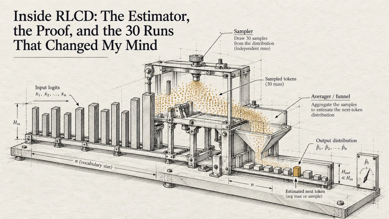
I went into this expecting the RL to be the interesting part. Laya's whole pitch is that a reinforcement-learning term turns noisy logits into calibrated probabilities, and the closed model it reproduces, Jev, is marketed on exactly that. My plan was to isolate the RL term, measure what it adds, and write it up as a win for reinforcement learning.

Thirty training runs later, the RL term is the most boring part of the pipeline. Here is the long version, with the math, the proof, and every table I generated.

Atomic answer: Laya's RL term is an evolution-strategies estimator of the gradient of a noise-smoothed proper scoring rule. As the noise vanishes it equals the cross-entropy gradient the model already has; at non-zero noise it provably makes the noise-free inference distribution over-sharp. Across CE-only, RL+CE, RL-only, a σ sweep to 4, a reward-weight sweep, and a reward-composition sweep, the RL term never improves accuracy, and CE-only is at least as good on every proper score.

TL;DR

• The RL gradient is −∇ L_rl = (1/(Gσ²)) Σ a_g ε_g, a group-baselined Monte Carlo estimate of ∇_z J_σ(z) with J_σ(z) = E_ε[R(softmax(z+ε), t)]. Stein's lemma turns it into a smoothed version of ∇R.

• For the log score, ∇R = t − softmax(z), so the RL term is a noisy estimator of the CE gradient. As σ → 0 they coincide.

• For σ > 0 the optimum satisfies E_ε[softmax(z*+ε)] = t, so the noise-free softmax(z*) is over-sharp. I prove the binary case with an explicit inequality.

• I verified the identity directly on trained models: at σ=2, the noise-averaged prediction lands on the target (gap −0.006) while noise-free inference is over-sharp (+0.108).

• 30 runs: nothing beats CE-only except a larger input token budget.

The estimator, written out

Each question is one sequence. A ModernBERT-large encoder runs over it, a type embedding is added, two pre-norm transformer layers mix the sequence, and an MLP scorer reads one logit z_i from the hidden state at each option's [MASK] marker. For a batch of B rows with K options, the training objective is

L = w_rl · L_rl + w_ce · L_ce

where L_ce is soft cross-entropy against the teacher's target t, and L_rl perturbs the logits:

ε_g ~ N(0, σ²), projected to zero mean over the valid options
q_g = softmax(z.detach() + ε_g)
r_g = R(q_g, t)                       # proper score
a_g = (r_g − mean_g r) / std(a)       # group-baselined advantage
L_rl = −mean_g a_g · log N(z+ε_g | z, σ²)

Define J_σ(z) = E_ε[R(softmax(z+ε), t)]. Since ∇_z log N(z+ε | z, σ²) = ε/σ², the gradient of L_rl is a Monte Carlo estimate of

∇_z J_σ(z) = (1/σ²) E[ R(softmax(z+ε), t) · ε ]  =  P · E[ ∇_u R(softmax(u), t) |_{u=z+ε} ]

The second equality is Stein's lemma, and it is the whole story: the RL gradient is the CE gradient averaged over logit noise. For the log score, ∇_u R = t − softmax(u). So as σ → 0, the RL term estimates t − softmax(z) — the negative CE gradient itself. It is a noisy proxy for something the CE term supplies exactly.

Why does this matter for calibration rather than just for elegance? Because the optimum of the smoothed objective is not the optimum of the unsmoothed one.

Why the smoothed optimum is over-sharp (and the binary proof)

For the log score, J_σ is concave (an average of concave log-softmax terms), so its maximisers satisfy the stationarity condition

E_ε[ softmax(z*_σ + ε) ] = t

The noise-averaged prediction equals the target. But inference runs at ε = 0 and reports the noise-free softmax(z*_σ). Averaging a softmax over noise flattens it, so the noise-free value must be sharper than the average. That's the over-confidence, and it's a property of the objective, not a training artefact.

For binary questions (noul, K=2) I can make it exact. With projected noise the logit gap d = z_1 − z_2 receives η ~ N(0, 2σ²), and stationarity becomes F_σ(d*) = E[s(d* + η)] = t_1 with s the logistic function.

Proposition. Let K=2, the log score, and t_1 ∈ (½, 1). For every σ > 0 there is a unique maximiser d*_σ. It satisfies s(d*_σ) > t_1, and s(d*_σ) is strictly increasing in σ.

The proof is a pairing argument. Let g = s − ½. It's odd, increasing, and concave on [0, ∞), with g''(x) = s(1−s)(1−2s) negative for x > 0. Fix d > 0 and pair ±η. If |η| ≤ d, concavity gives g(d+η) + g(d−η) ≤ 2g(d). If |η| > d, use oddness to rewrite the pair as g(|η|+d) − g(|η|−d) — the increment of a concave function over an interval of length 2d, which is at most g(2d) ≤ 2g(d). So E[g(d+η)] < g(d), hence F_σ(d) < s(d) for all d > 0. Since F_σ is continuous and strictly increasing from ½ to 1, it has a unique root d*, and s(d*) > F_σ(d*) = t_1. For monotonicity, write η = τZ; Stein's lemma gives ∂_τ E[g(d+τZ)] = τ E[g''(d+τZ)] < 0, so F_σ decreases in σ at fixed d, and keeping F_σ(d*_σ) = t_1 forces d*_σ up.

A second-order expansion adds the size: E[softmax(z+ε)] = softmax(z) + (σ²/2) Σ P_jk ∂_j∂_k softmax(z) + O(σ⁴). The bias is O(σ²) — negligible at Laya's annealed σ ≤ 0.4, large at σ = 2. That predicts Laya's recipe is nearly unbiased and gains nothing over CE, which is exactly what the runs show.

Direct check: average the noise away and watch it hit the target

The proposition is about the objective's optimum. The trained checkpoints let me check it end to end. For each fixed-σ model I compared, over the full 2,000-decision test set, the noise-free softmax(z*) with a 128-sample average E_ε[softmax(z*+ε)].

At σ=2 the noise-averaged prediction lands on the target — the gap is −0.006, essentially zero — while the noise-free prediction that inference reports is over-sharp by +0.108. Averaging moves 68% of rows toward the target. This is the smoothest confirmation of the theory I got, and it took one inference pass plus noise samples.

The full σ sweep

I extended the original sweep to σ ∈ {0.25, 0.5, 1, 2, 3, 4}, three seeds up to σ=2.

Fitted temperature and NLL rise monotonically across the whole range. The sharpness gap rises, then saturates as the softmax runs out of room. Accuracy is flat within seed noise — the RL term is not buying accuracy, it is buying sharpness, and only at inference.

Reward weight and reward composition

Two more sweeps to make sure I wasn't missing a working configuration.

At fixed σ=1, scaling the RL weight while holding CE fixed does what the cancellation argument predicts: accuracy flat, proper scores worse as the RL term grows.

And the reward composition — log-only vs log+spherical vs log+RPS, under Laya's schedule:

No reward term earns its place. The spherical and RPS additions are inside seed noise on accuracy and don't move Brier at all.

Gradient diagnostics: big and misaligned

I logged the cosine and norm ratio between the RL and CE gradients w.r.t. the logits every ten steps. Under Laya's schedule the RL gradient is 8× the CE gradient at σ=0.4 and 87× at σ=0.1, with cosine around 0.65. In the fixed-σ runs, where σ isn't confounded with training progress, the norm ratio scales as 1/σ and alignment falls from 0.60 to 0.37 as σ grows.

So the RL term dominates the update before clipping, and points only moderately the same way as CE. It's not a gentle regulariser; it's the loudest signal in the loss, and it's a noisy copy of a signal already present.

Consistency probes

A practical question the calibration numbers don't answer: does the model behave the same when the surface form changes? On the σ=2 checkpoint, 500 questions:

Option order and renaming are mostly handled. Unrelated context is not — 13% of picks flip when you pad the state, the same fragility TypeSafe documents for Jev. A rough negation probe (negate the instruction, swap true/false) leaves a mean mismatch of 0.53 between the two wordings, which is a lot; but that probe is crude, and I'd treat it as a flag rather than a number.

The one thing that moved accuracy

Every loss-side knob plateaued at ~0.78. Then I read the checkpoint card carefully: it documents a 1024-token context and a 256-token option budget, and warns that a large option set starves each option of tokens. My port had been built at 512/192. Matching the documented budget gave the only real gain:

Continuing from the already fine-tuned laya-typed-decisions checkpoint gave the same result, so the gain is the budget, not the starting point. It also means the loss ablation was being run slightly under-provisioned for the option-rich questions.

What I'd do differently, and what's still open

• Try a CE+Brier composite loss. Verdict-2.0, a 151M ModernBERT-base decision model, reports 0.771 accuracy with ECE 0.0144 on this exact benchmark using a cross-entropy plus Brier objective. I didn't test it; it's the most obvious next run.

• Report seeds. I ran three seeds where I could afford it. Small accuracy gaps move as much as a modest architecture change when you pick a different seed, so I never compare models by single-seed accuracy.

• Stop treating the RL term as the interesting variable. The interesting variable was the input budget. I'd start there next time.

How to reproduce

All code, configs, and per-run JSON are in LakoreAI/sev.

If you've built a typed-decision model and checked your fitted temperature, I want to know what it came out to. Mine was always greater than 1, and I suspect yours is too.

Follow me: LinkedIn | GitHub